How to Simulate Past Investments Like a Pro
A practical expert guide to backtesting portfolios with clean data, explicit assumptions, DCA vs lump sum comparisons, fees, rebalancing, risk metrics, and charts investors can actually understand.
Bad prices, missing dividends, currency mismatches, or survivor bias can make a backtest look better than reality.
Contribution dates, fees, execution prices, rebalancing rules, and risk metrics must be explicit before comparing results.
CAGR is useful, but drawdowns, recovery time, volatility, and rolling returns explain whether a strategy is livable.
Why Learning to Simulate Past Investments Matters
Learning how to simulate past investments helps investors move from vague opinions to measurable tradeoffs. Instead of asking whether an ETF, stock, or crypto asset “feels” attractive, you can test how a strategy would have behaved across market cycles, crashes, rebounds, and long boring stretches.
A useful backtest does not predict the future. It helps you understand the range of outcomes that happened under real historical stress. That is valuable because most investment mistakes are not spreadsheet mistakes. They are expectation mistakes. Investors abandon strategies when the actual ride feels more painful than the version they imagined.
A professional simulation should answer practical questions: what would have happened if I invested every month, how much did the portfolio fall, how long did it take to recover, did lump sum beat DCA, how sensitive were the results to the start date, and what assumptions changed the outcome?
Data Quality: The Foundation of Every Backtest
The quality of an investment simulator depends on the quality of its data. If the historical prices are incomplete or inconsistent, the final chart can look precise while being wrong. This is especially important for ETFs, dividend-paying assets, crypto, international holdings, and portfolios that mix currencies.
For stocks and ETFs, adjusted prices are usually better than raw prices because they account for splits and distributions. For crypto, the challenge is different: markets trade continuously, so you need clear rules for daily close time, exchange source, and missing data. For international assets, exchange rates can materially change the investor’s real result.
| Data issue | Why it matters | Cleaner approach |
|---|---|---|
| Missing dividends | Understates total return for income assets. | Use adjusted close or total return data when available. |
| Survivorship bias | Only including winners makes strategies look safer. | Include delisted assets when testing broad historical universes. |
| Currency mismatch | Returns can change after FX conversion. | Define base currency and convert consistently. |
| Different calendars | Stocks, ETFs, and crypto do not share identical trading schedules. | Align dates before calculating portfolio values. |
Useful external sources include Yahoo Finance, CoinGecko, Alpha Vantage, and FRED.
Assumptions You Must Define Before Running Results
Every backtest is a model, and every model has assumptions. The problem is not having assumptions. The problem is hiding them. Before you compare DCA, lump sum, rebalancing, or different ETFs, define the rules clearly enough that someone else could reproduce the same result.
Investment assumptions
- Initial amount and recurring contribution amount.
- Contribution frequency: weekly, bi-weekly, monthly, or yearly.
- Start date and end date.
- Asset list, weights, and base currency.
- Dividend reinvestment rule.
Execution assumptions
- Buy at close, open, average price, or a fixed monthly date.
- Transaction fees and spreads.
- ETF expense ratio or management fee drag.
- Tax treatment if relevant.
- Rebalancing calendar or threshold.
A small assumption can change the conclusion. A simulation that buys at the lowest price of each month is not realistic. A simulation that ignores dividends can penalize income ETFs. A simulation that excludes fees can exaggerate high-turnover strategies. Professional backtesting is less about making a chart and more about making the rules honest.
A Professional Workflow to Simulate Past Investments
A reliable workflow separates data, rules, calculation, analytics, and presentation. This prevents the simulator from becoming a black box where the user sees a result but cannot understand how it was built.
- Collect data: choose sources, download historical prices, verify date ranges, and preserve raw files.
- Clean and align: remove duplicates, handle missing values, adjust for splits or dividends, and align calendars.
- Define parameters: contribution schedule, lump sum amount, fees, asset allocation, rebalancing, and base currency.
- Run the engine: calculate units purchased, cash balance, portfolio value, contributions, and returns through time.
- Compute metrics: CAGR, total return, max drawdown, recovery time, volatility, rolling returns, and hit ratio.
- Visualize results: show portfolio value, contributions, drawdowns, rolling returns, and strategy comparison.
- Interpret carefully: explain what the simulation shows, what it does not show, and which assumptions drive the result.
DCA vs Lump Sum Backtesting
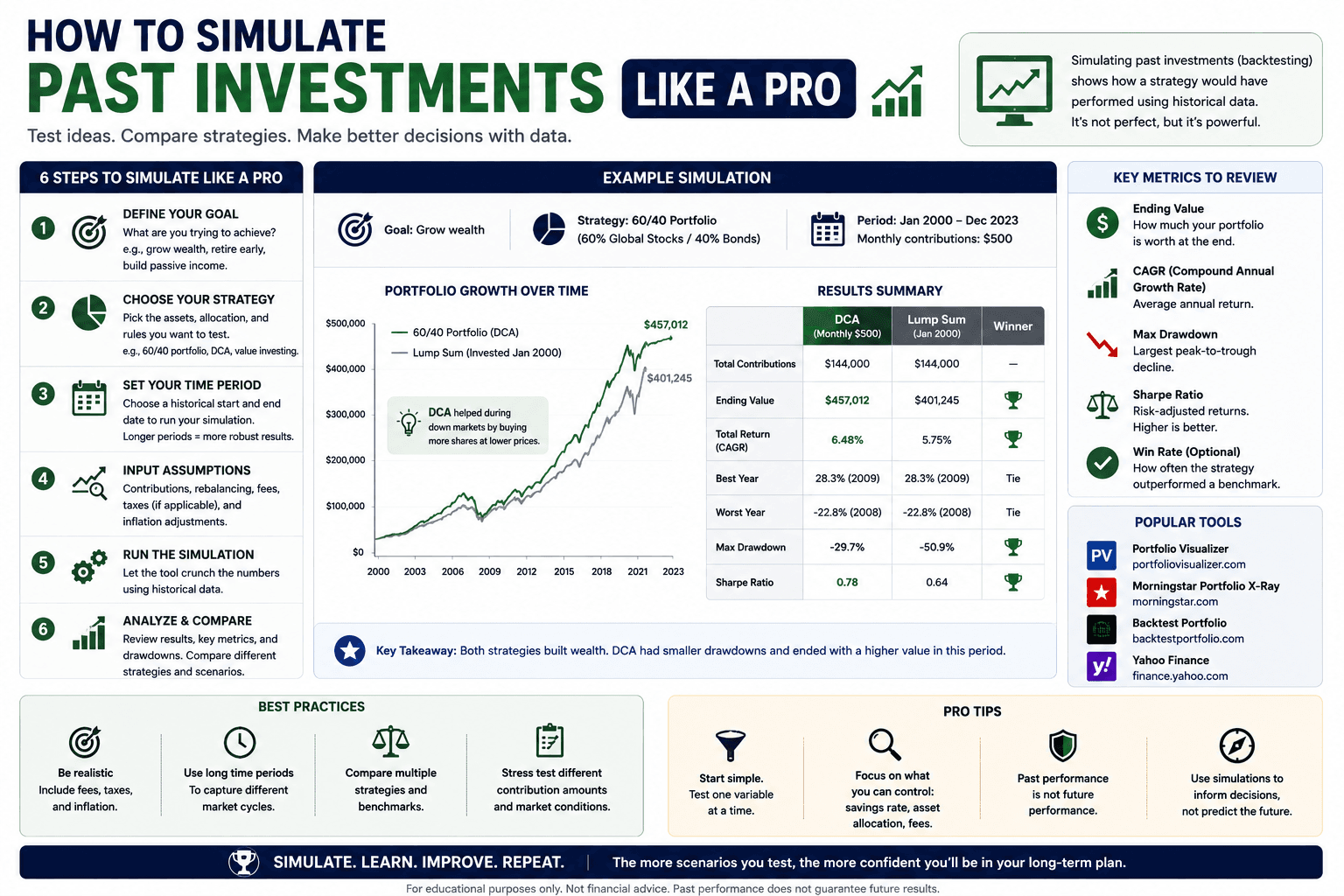
One of the most common reasons people simulate past investments is to compare dollar-cost averaging with lump sum investing. Lump sum puts all capital to work immediately. DCA spreads the entry across time. The historical winner depends heavily on market trend, start date, asset volatility, and the investor’s emotional tolerance.
In long rising markets, lump sum often has an advantage because more money spends more time invested. During sharp declines or uncertain entry periods, DCA can reduce regret and lower the risk of investing everything right before a fall. That does not make DCA mathematically superior in every case. It makes DCA behaviorally useful for many real investors.
// Minimal DCA logic
function simulateDCA(prices, contribution) {
  let units = 0;
  return prices.map(row => {
    units += contribution / row.close;
    return { date: row.date, value: units * row.close };
  });
}

// Minimal lump sum logic
function simulateLumpSum(prices, initialAmount) {
  const units = initialAmount / prices[0].close;
  return prices.map(row => ({ date: row.date, value: units * row.close }));
}
For a deeper strategy comparison, connect this article to DCA vs Lump Sum: When One Clearly Wins and the DCA Calculator.
Fees, Slippage, Taxes, and Rebalancing
A backtest that ignores costs is often too optimistic. Even small costs can matter across hundreds of recurring contributions. This is especially true when simulating weekly investing, multi-asset rebalancing, small account balances, or assets with wide spreads.
For ETFs, expense ratios are usually embedded in fund performance, but if you are modeling raw index returns or synthetic portfolios, you may need to subtract an annual drag. For stocks and crypto, spreads and liquidity can matter more than the headline commission. For taxable accounts, selling to rebalance can create tax events, so cash-first rebalancing may be more realistic.
| Friction | How to model it | Why it matters |
|---|---|---|
| Fixed fee | Subtract a dollar amount per trade. | Hurts small frequent contributions. |
| Percentage fee | Subtract a percent of trade value. | Scales with position size. |
| Slippage | Buy slightly above reference price, sell slightly below. | More realistic for illiquid assets. |
| Rebalancing | Calendar, threshold, or cash-first rules. | Controls risk but can create trades. |
Risk Metrics That Matter More Than Final Value
The final portfolio value is only one part of the story. A strategy can end with a strong result but still be emotionally impossible for many investors to hold. That is why a good investment simulator should show risk metrics alongside return metrics.
Return metrics
- Total return: overall gain or loss.
- CAGR: annualized compound growth rate.
- XIRR: useful when contributions happen on irregular dates.
- Rolling returns: shows how results vary across start dates.
Risk metrics
- Max drawdown: worst peak-to-trough decline.
- Recovery time: months or years to regain the prior high.
- Volatility: variability of returns.
- Sharpe or Sortino: risk-adjusted return measures.
For user experience, drawdown charts are powerful because they show the pain period directly. A smooth-looking portfolio value chart can hide how long the investor spent underwater. A drawdown chart makes that reality visible.
Visualization and UX: Turn Data Into Decisions
The best investment simulators do not simply output a number. They help users understand the result. A strong interface should show portfolio growth, total contributions, interest or gains, drawdowns, rolling returns, and a clear comparison between strategies.
Charts should be readable on mobile. Tooltips should show dates, values, contributions, and drawdowns. Tables should be scrollable. Labels should explain what each metric means without overwhelming the user. The goal is to make the next decision easier: invest now, DCA over time, change allocation, reduce risk, or test another scenario.
- Use line charts for portfolio value and strategy comparison.
- Use area charts to separate contributions from growth.
- Use drawdown charts to show risk clearly.
- Use tables for yearly breakdowns and exportable details.
- Use presets so beginners can test common assets quickly.
This is also where internal linking matters. Readers who understand the method should move naturally into the Portfolio Backtester, DCA Calculator, or backtesting guide.
Practical Simulation Scenarios Worth Testing
A useful simulator should not test only one perfect scenario. It should let the investor compare multiple realistic situations. This is where many simple calculators fall short: they show one final number, but they do not explain how fragile that number is. A stronger workflow tests the same strategy across different dates, contribution schedules, market regimes, and asset mixes.
The first scenario to test is a normal long-term DCA plan. For example, a monthly contribution into a broad-market ETF can show how consistent investing behaves through growth periods and downturns. The goal is not to find the highest possible return. The goal is to understand the range of outcomes an ordinary investor might actually live through.
The second scenario is a bad-timing lump sum. This helps the investor understand sequence risk. If the portfolio falls soon after investing, how deep is the drawdown, and how long does recovery take? This test is valuable because many people can accept volatility in theory but struggle when losses happen immediately after they invest.
The third scenario is a delayed-entry strategy. Some investors wait in cash because markets feel expensive. A simulator can test the opportunity cost of waiting. Sometimes waiting avoids a decline. Other times it misses gains. The point is not to shame caution, but to measure what caution historically cost under different conditions.
The fourth scenario is diversification. Compare a single equity ETF with a balanced portfolio, an all-in-one ETF, or a portfolio that includes bonds, international equities, or cash. The ending value may not always be highest, but the drawdown and recovery profile can be better. For many investors, the best portfolio is not the one with the highest historical return; it is the one they can hold without panicking.
| Scenario | Question it answers | Useful metric |
|---|---|---|
| Monthly DCA | What happens if I invest consistently? | Ending value, total contributions, rolling returns |
| Bad-timing lump sum | What if I invest right before a downturn? | Max drawdown, recovery time |
| Delayed entry | What is the cost of waiting in cash? | Opportunity cost, missed upside |
| Diversified portfolio | Does lower volatility improve the experience? | Drawdown, volatility, risk-adjusted return |
Common Mistakes When Simulating Past Investments
Backtesting can create false confidence when it is done carelessly. The most dangerous simulations are the ones that look professional but quietly rely on unrealistic assumptions.
- Cherry-picking dates: choosing a lucky start date can make almost any strategy look brilliant.
- Ignoring bad periods: a robust test should include crashes, sideways markets, and recoveries.
- Using price return instead of total return: this can distort dividend ETF comparisons.
- Forgetting taxes and fees: especially harmful for high-turnover strategies.
- Overfitting: tuning parameters to one historical period may fail in the next one.
- Confusing hindsight with skill: knowing the best asset after the fact is not an investable strategy.
How This Supports Better Investing Decisions
When used correctly, historical simulation helps investors choose a process they can actually follow. It can reveal that a strategy with the highest ending value also had an unacceptable drawdown. It can show that DCA produced lower regret even when lump sum had stronger returns. It can highlight that diversification reduced recovery time, even if it slightly reduced upside.
This is the kind of decision support that builds trust. A reader who lands on this article should leave with a clear understanding of the methodology and a natural reason to use your tools. That makes this page a strong SEO pillar for the entire investing simulator cluster.
How to Interpret Results Without Overreacting
The most important part of a simulation is not the chart itself. It is the interpretation. A backtest can show that one strategy won historically, but the investor still has to ask whether that result came from a durable principle or from a lucky period. This distinction matters because a strategy that looks perfect in one historical window can disappoint badly in another.
Start by checking whether the winning strategy won by a large margin or a tiny margin. A small advantage may disappear after fees, taxes, slippage, or a slightly different contribution date. Next, review whether the strategy required behavior that would have been hard to maintain. If a strategy only worked because the investor held through a severe drawdown without changing anything, that must be acknowledged.
Then compare results across several start dates. If a strategy works only from one carefully chosen date, it may be fragile. Rolling windows are useful because they show how the result changes when the start month moves forward. This is one of the best ways to avoid cherry-picking and build a more honest view of the strategy.
Finally, connect the simulation to the investor’s actual financial life. A young investor with stable income may be comfortable with larger drawdowns. A retiree or short-term saver may care more about capital preservation and recovery time. The same backtest can lead to different conclusions for different people because goals, timelines, and cash flow are different.
Frequently Asked Questions
What does it mean to simulate past investments?
It means using historical data to model how a portfolio, contribution schedule, or investment strategy would have behaved over a past period.
Is backtesting the same as predicting future returns?
No. Backtesting studies historical behavior. It can improve expectations and risk awareness, but it does not guarantee future performance.
What is the easiest strategy to backtest first?
DCA versus lump sum is a useful starting point because it is easy to understand and directly relevant for most long-term investors.
Which metric should I look at first?
Start with final value and CAGR, then immediately review max drawdown, recovery time, and rolling returns. The risk path matters as much as the endpoint.
Can I simulate ETFs, stocks, and crypto?
Yes, but each asset type needs clean data and consistent rules. Crypto requires extra care because it trades continuously and can have different price sources.
Why do different simulators show different results?
They may use different data sources, adjusted prices, contribution dates, fee assumptions, dividend rules, or rebalancing methods.